LESSON 1: ROOTS OF ALGEBRAIC AND TRANSCENDENTAL EQUATION

Root-finding algorithm

-is a numerical method, or algorithm, for finding a value x such that f(x) = 0, for a given function f. Such an x is called a root of the function f.

This article is concerned with finding scalar, real or complex roots, approximated as floating point numbers. Finding integer roots or exact algebraic roots are separate problems, whose algorithms have little in common with those discussed here. (See: Diophantine equation as for integer roots)

Finding a root of f(x) − g(x) = 0 is the same as solving the equation f(x) = g(x). Here, x is called the unknown in the equation. Conversely, any equation can take the canonical form f(x) = 0, so equation solving is the same thing as computing (or finding) a root of a function.

Numerical root-finding methods use iteration, producing a sequence of numbers that hopefully converge towards a limit (the so called "fixed point") which is a root. The first values of this series are initial guesses. The method computes subsequent values based on the old ones and the function f.

The behaviour of root-finding algorithms is studied in numerical analysis. Algorithms perform best when they take advantage of known characteristics of the given function. Thus an algorithm to find isolated real roots of a low-degree polynomial in one variable may bear little resemblance to an algorithm for complex roots of a "black-box" function which is not even known to be differentiable. Questions include ability to separate close roots, robustness in achieving reliable answers despite inevitable numerical errors, and rate of convergence.

Specific algorithms

The simplest root-finding algorithm is the bisection method. It works when f is a continuous function and it requires previous knowledge of two initial guesses, a and b, such that f(a) and f(b) have opposite signs. Although it is reliable, it converges slowly, gaining one bit of accuracy with each iteration.

Newton's method assumes the function f to have a continuous derivative. Newton's method may not converge if started too far away from a root. However, when it does converge, it is faster than the bisection method, and is usually quadratic. Newton's method is also important because it readily generalizes to higher-dimensional problems. Newton-like methods with higher order of convergence are the Householder's methods. The first one after Newton's method is Halley's method with cubic order of convergence.

Replacing the derivative in Newton's method with a finite difference, we get the secant method. This method does not require the computation (nor the existence) of a derivative, but the price is slower convergence (the order is approximately 1.6).

The false position method, also called the regula falsi method, is like the secant method. However, instead of retaining the last two points, it makes sure to keep one point on either side of the root. The false position method is faster than the bisection method and more robust than the secant method, but requires the two starting points to bracket the root.

The secant method also arises if one approximates the unknown function f by linear interpolation. When quadratic interpolation is used instead, one arrives at Müller's method. It converges faster than the secant method. A particular feature of this method is that the iterates x_n may become complex.

This can be avoided by interpolating the inverse of f, resulting in the inverse quadratic interpolation method. Again, convergence is asymptotically faster than the secant method, but inverse quadratic interpolation often behaves poorly when the iterates are not close to the root.

Finally, Brent's method is a combination of the bisection method, the secant method and inverse quadratic interpolation. At every iteration, Brent's method decides which method out of these three is likely to do best, and proceeds by doing a step according to that method. This gives a robust and fast method, which therefore enjoys considerable popularity.

Finding multiple roots

If p(x) is a polynomial with a multiple root at r, then finding the value of r can be difficult (inefficient or impossible) for many of the standard root-finding algorithms. Fortunately, there is a technique especially for this case, provided that p is given explicitly as a polynomial in one variable with exact coefficients.

Algorithm

1. First, we need to determine whether p(x) has a multiple root. If p(x) has a multiple root at r, then its derivative p′(x) will also have a root at r (one fewer than p(x) has there). So we calculate the greatest common divisor of the polynomials p(x) and p′(x); adjust the leading coefficient to be one and call it g(x). (See Sturm's theorem.) If g(x) = 1, then p(x) has no multiple roots and we can safely use those other root-finding algorithms which work best when there are no multiple roots, and then exit.
2. Now suppose that there is a multiple root. Notice that g(x) will have a root of the same multiplicity at r that p′(x) has and the degree of the polynomial g(x) will generally be much less than that of p(x). Recursively call this routine, i.e. go back to step #1 above, using g(x) in place of p(x). Now suppose that we have found the roots of g(x), i.e. we have factored it.
3. Since r has been found, we can factor (x−r) out of p(x) repeatedly until we have removed all of the roots at r. Repeat this for any other multiple roots until there are no more multiple roots. Then the quotient, i.e. the remaining part of p(x), can be factored in the usual way with one of the other root-finding algorithms. Exit.

Example

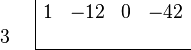
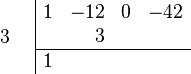
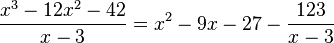
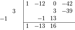
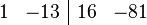
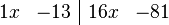
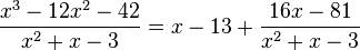
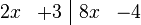
Suppose p(x) = x³+x²−5x+3 is the function whose roots we want to find. We calculate p′(x) = 3x²+2x−5. Now divide p′(x) into p(x) to get p(x) = p′(x)·((1/3)x+(1/9))+((−32/9)x+(32/9)). Divide the remainder by −32/9 to get x−1 which is monic. Divide x−1 into p′(x) to get p′(x) = (x−1)·(3x+5)+0. Since the remainder is zero, g(x) = x−1. So the multiple root of p(x) is r = 1. Dividing p(x) by (x−1)², we get p(x) = (x+3)(x−1)² so the other root is −3, a single root.

Algebraic geometry

The performance of standard polynomial root-finding algorithms degrades in the presence of multiple roots. Using ideas from algebraic geometry, Zhonggang Zeng has published a more sophisticated approach, with a MATLAB package implementation, that identifies and handles multiplicity structures considerably better. A different algebraic approach including symbolic computations has been pursued by Andrew Sommese and colleagues, available as a preprintPDF). (

Direct algorithm for multiple root elimination

There is a direct method of eliminating multiple (or repeated) roots from polynomials with exact coefficients (integers, rational numbers, Gaussian integers or rational complex numbers).

Suppose a is a root of polynomial P, with multiplicity m>1. Then a will be a root of the formal derivative P ’, with multiplicity m−1. However, P ’ may have additional roots that are not roots of P. For example, if P(x)=(x−1)³(x−3)³, then P ’(x)=6(x−1)²(x−2)(x−3)². So 2 is a root of P ’, but not of P.

Define G to be the greatest common divisor of P and P ’. (Say, G(x) = (x−1)²(x−3)²).

Finally, G divides P exactly, so form the quotient Q =P/G. (Say, Q(x)= (x−1)(x−3) ). The roots of Q are the multiple roots of P.

As P is a polynomial with exact coefficients, then if the algorithm is executed using exact arithmetic, Q will also be a polynomial with exact coefficients.

Obviously degree(Q) <>P). If degree(Q) ≤ 4 then the multiple roots of P may be found algebraically. It is then possible to determine the multiplicities of those roots in P algebraically.

Iterative root-finding algorithms perform well in the absence of multiple roots.

Transcendental Equation

A transcendental equation is an equation containing a transcendental function. Examples of such an equation are

x = e ^{− x}

x = sin(x)

Solution methods

Some methods of finding solutions to a transcendental equation use graphical or numerical methods. For a graphical solution, one method is to set each side of a single variable transcendental equation equal to a dependent variable (for example, y) and plot the two graphs, using their intersecting points to find solutions. The numerical solution extends from finding the point at which the intersections occur using some kind of numerical calculations (calculator or math software). Approximations can also be made by truncating the Taylor series if the variable is considered to be small. Additionally, Newton's method could be used to solve the equation.

Often special functions can be used to write the solutions to transcendental equations in closed form. In particular, the first equation has a solution in terms of the Lambert W Function.

LESSON 1: A. Incremental Search

Incremental search

Incremental search has been studied at least since the late 1960s. Incremental search algorithms reuse information from previous searches to speed up the current search and solve search problems potentially much faster than solving them repeatedly from scratch.^[1] Similarly, heuristic search has been studied at least since the late 1960s. Heuristic search algorithms, often based on A*, use heuristic knowledge in the form of approximations of the goal distances to focus the search and solve search problems potentially much faster than uninformed search algorithms.Incremental heuristic search algorithms combine both incremental and heuristic search to speed up searches of sequences of similar search problems, which is important in domains that are only incompletely known or change dynamically.The resulting search problems, sometimes called dynamic path planning problems, are graph search problems where paths have to be found repeatedly because the topology of the graph, its edge costs, the start vertex or the goal vertices change over time.

So far, three main classes of incremental heuristic search algorithms have been developed:

• The first class restarts A* at the point where its current search deviates from the previous one (example: Fringe Saving A*).

• The second class updates the h-values from the previous search during the current search to make them more informed (example: Generalized Adaptive A*).

• The third class updates the g-values from the previous search during the current search to correct them when necessary, which can be interpreted as transforming the A* search tree from the previous search into the A* search tree for the current search (examples: Lifelong Planning A*, D*, D* Lite).

All three classes of incremental heuristic search algorithms are different from other replanning algorithms, such as planning by analogy, in that their plan quality does not deteriorate with the number of replanning episodes.

Applications

Incremental heuristic search has been extensively used in robotics, where a larger number of path planning systems are based on either D* (typically earlier systems) or D* Lite (current systems), two different incremental heuristic search algorithms.

LESSON 1: B. Bisection and False Methods

Nonlinear Equations: Bisection Method : Background : Youtube

Nonlinear Equations: Bisection Method : Algorithm : Youtube

Nonlinear Equations: Bisection Method : Example : Youtube

Assessment Bisection Method Nonlinear Equation

LESSON 2: NEWTON-RAPHSON AND SECANT METHODS

Newton-Raphson Method

Nonlinear Equations: Nonlinear Equations : Derivation : Youtube

Nonlinear Equations: Newton Raphson Method : Example : Youtube

Nonlinear Equations: Secant Method : Derivation Approach 1 : Youtube

Nonlinear Equations: Secant Method : Derivation Approach 2 : Youtube

Nonlinear Equations: Secant Method : Algorithm : Youtube

Nonlinear Equations: Secant Method : Example : Youtube

Assessment - Nonlinear - Secant Method

LESSON 3: ROOTS OF POLYNOMIALS

Finding roots of polynomials

Much attention has been given to the special case that the function f is a polynomial; there exist root-finding algorithms exploiting the polynomial nature of f. For a univariate polynomial of degree less than five, we have closed form solutions such as the quadratic formula. However, even this degree-two solution should be used with care to ensure numerical stability, the degree-four solution is unwieldy and troublesome. Higher-degree polynomials have no such general solution, according to the Abel–Ruffini theorem (1824, 1799).

For real roots, Sturm's theorem provides a guide to locating and separating roots. This plus interval arithmetic combined with Newton's method yields a robust algorithm, but other choices are more common.

One possibility is to form the companion matrix of the polynomial. Since the eigenvalues of this matrix coincide with the roots of the polynomial, one can use any eigenvalue algorithm to find the roots of the polynomial. For instance the classical Bernoulli's method to find the root greater in modulus, if it exists, turns out to be the power method applied to the companion matrix. The inverse power method, which finds some smallest root first, is what drives the Jenkins–Traub method and gives it its numerical stability and fast convergence even in the presence of multiple or clustered roots.

Laguerre's method, as well as Halley's method, use second order derivatives and complex arithmetics, including the complex square root, to exhibit cubic convergence for simple roots, dominating the quadratic convergence displayed by Newton's method.

Bairstow's method uses Newton's method to find quadratic factors of a polynomial with real coefficients. It can determine both real and complex roots of a real polynomial using only real arithmetic.

The simple Durand–Kerner and the slightly more complicated Aberth method simultaneously finds all the roots using only simple complex number arithmetic.

The splitting circle method is useful for finding the roots of polynomials of high degree to arbitrary precision; it has almost optimal complexity in this setting. Another method with this style is the Dandelin–Gräffe method (actually due to Lobachevsky) which factors the polynomial.

Wilkinson's polynomial illustrates that high precision may be necessary when computing the roots of a polynomial.

LESSON 4: SYNTHETIC DIVISION

Synthetic division

Synthetic division is a method of performing polynomial long division, with less writing and fewer calculations. It is mostly taught for division by binomials of the form

but the method generalizes to division by any monic polynomial. This method can be used instead of long division on integers by considering 10 = x and only substituting 10 back in at the end.

The most useful aspect of synthetic division is that it allows one to calculate without writing variables using fewer calculations. As well, it takes significantly less space than long division. Most importantly, the subtractions in long division are converted to additions by switching the signs at the very beginning, preventing sign errors.

Synthetic division for linear denominators is also called division through Ruffini's rule.

Regular Synthetic Division

The first example is Synthetic Division with only a monic linear denominator x − a .

Write the coefficients of the polynomial to be divided at the top (the zero is for the unseen 0x).

Negate the coefficients of the divisor.

Write in every coefficient of the divisor but the first one on the left.

Note the change of sign from −3 to 3. "Drop" the first coefficient after the bar to the last row.

Multiply the dropped number by the number before the bar, and place it in the next column.

Perform an addition in the next column.

Repeat the previous two steps and the following is obtained

Count the terms to the left of the bar. Since there is only one, the remainder has degree one. Mark the separation with a vertical bar.

The terms are written with increasing degree from right to left beginning with degree zero for both the remainder and the result.

The result of the division is:

Expanded Synthetic Division

This method works for bigger divisors with only a slight modification with changes in bold. Using the same steps as before, let's try to perform the following division:

We concern ourselves only with the coefficients. Write the coefficients of the polynomial to be divided at the top.

Negate the coefficients of the divisor.

Write in every coefficient but the first one on the left in an upward right diagonal (see next diagram).

Note the change of sign from 1 to −1 and from −3 to 3 . "Drop" the first coefficient after the bar to the last row.

Multiply the dropped number by the diagonal before the bar, and place the resulting entries diagonally to the right from the dropped entry.

Perform an addition in the next column.

Repeat the previous two steps until you would go past the entries at the top with the next diagonal.

Then simply add up any remaining columns.

Count the terms to the left of the bar. Since there are two, the remainder has degree two. Mark the separation with a vertical bar.

The terms are written with increasing degree from right to left beginning with degree zero for both the remainder and the result.

The result of our division is:

For non-monic divisors

With a little prodding, the expanded technique may be generalised even further to work for any polynomial, not just monics. The usual way of doing this would be to divide the divisor g(x) with its leading co-efficient (call it a)

then using synthetic division with h(x) as the divisor, and then multiplying the remainder by a to get the remainder of the original division (the quotient stays the same). But this often produces unslightly fractions which get removed later, and is thus more prone to error. It is possible to do it without first dividing the co-efficients of g(x) by a.

As can be observed by first performing long division with such a non-monic divisor, the co-efficients of f(x) are divided by the leading co-efficient of g(x) after "dropping", and before multiplying.

Let's illustrate by performing the following division:

A slightly modified table is used:

Note the extra row at the bottom. This is used to write values found by dividing the "dropped" values by the leading co-efficient of g(x) (in this case, indicated by the /3; note that, unlike the rest of the co-efficients of g(x), the sign of this number is not changed).

Next, the first co-efficient of f(x) is dropped as usual:

and then the dropped value is divided by 3 and placed in the row below:

Next, the new (divided) value is used to fill the top rows with multiples of 2 and 1, as in the expanded technique:

The 5 is dropped next, with the obligatory adding of the 4 below it, and the answer is divided again:

Then the 3 is used to fill the top rows:

At this point, if, after getting the third sum, we were to try and use it to fill the top rows, we would "fall off" the right side, thus the third value is the first co-efficient of the remainder, as in regular synthetic division. But the vaules of the remainder are not divided by the leading co-efficient of the divisor:

Now we can read of the co-efficients of the answer. As in expanded synthetic division, the last two values (2 is one less than the co-efficient of the divisor) are the co-efficients of the remainder, and the remaining values are the co-efficients of the quotient:

and the result is

LESSON 5: SCALING OF POLYNOMIALS

The Projector Method

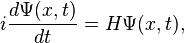
To motivate the algorithm, let's look at the Schrödinger equation for a particle in some potential in one dimension: We can condense the notation a bit by writing it in terms of an operator equation, with . So then we have where we have to keep in mind that H is an operator, not a simple number or function. There are special functions, called eigenfunctions, for which HΨ(x) = EΨ(x), where E is a number. These functions are special because no matter where we evaluate the action of the H operator on the wave function, we always get the same number E. These functions are called stationary states, because the time derivative at any point x is always the same, so the amplitude of the wave function never changes in time. Since the overall phase of a wave function is not measurable, the system does not change in time.

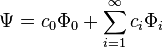
We are usually interested in the wave function with the lowest energy eigenvalue, the ground state. We're going to write a slightly different version of the Schrödinger equation that will have the same energy eigenvalue, but, instead of being oscillatory, it will be convergent. Here it is: . We've removed the imaginary number from the time derivative and added in a constant offset of E₀, which is the ground state energy. We don't actually know the ground state energy, but there will be a way to determine it self-consistently which we'll introduce later. Our modified equation(some people call it the imaginary-time Schrödinger equation) has some nice properties. The first thing to notice is that if we happen to guess the ground state wave function, then HΦ₀(x) = E₀Φ₀(x) and the time derivative is zero. Now suppose that we start with another wave function(Ψ), which is not the ground state but is not orthogonal to it. Then we can write it as a linear sum of eigenfunctions: Since this is a linear differential equation, we can look at the action of each part separately. We already determined that Φ₀ is stationary. Suppose we take Φ₁. Since Φ₀ is the lowest-energy eigenfunction, the associate eigenvalue of Φ₁ satisfies the property E₁ > E₀. Thus the time derivative of c₁ is negative, and will eventually go to zero, leaving us with only the ground state. This observation also gives us a way to determine E₀. We watch the amplitude of the wave function as we propagate through time. If it increases, then decrease the estimation of the offset energy. If the amplitude decreases, then increase the estimate of the offset energy.

Stochastic Implementation

Now we have an equation that, as we propagate it forward in time and adjust E₀ appropriately, we find the ground state of any given Hamiltonian. This is still a harder problem than classical mechanics, though, because instead of propagating single positions of particles, we must propagate entire functions. In classical mechanics, we could simulate the motion of the particles by setting x(t + τ) = x(t) + τv(t) + 0.5F(t)τ², if we assume that the force is constant over the time span of τ. For the imaginary time Schrödinger equation, instead, we propagate forward in time using a convolution integral with a special function called a Green's function. So we get . 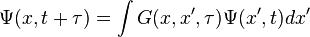Similarly to classical mechanics, we can only propagate for small slices of time; otherwise the Green's function is inaccurate. As the number of particles increases, the dimensionality of the integral increases as well, since we have to integrate over all coordinates of all particles. We can do these integrals by Monte Carlo integration.