Gauss–Seidel method
From Wikipedia, the free encyclopedia
In numerical linear algebra, the Gauss–Seidel method, also known as the Liebmann method or the method of successive displacement, is an iterative method used to solve a linear system of equations. It is named after the German mathematicians Carl Friedrich Gauss and Philipp Ludwig von Seidel, and is similar to the Jacobi method. Though it can be applied to any matrix with non-zero elements on the diagonals, convergence is only guaranteed if the matrix is either diagonally dominant, or symmetric and positive definite.
Description
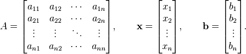
Given a square system of n linear equations with unknown x:

where:
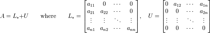
Then A can be decomposed into a lower triangular component L*, and a strictly upper triangular component U:
The system of linear equations may be rewritten as:

The Gauss–Seidel method is an iterative technique that solves the left hand side of this expression for x, using previous value for x on the right hand side. Analytically, this may be written as:

However, by taking advantage of the triangular form of L*, the elements of x(k+1) can be computed sequentially using forward substitution:
i}a_{ij}x^{(k)}_j - \sum_{j
Note that the sum inside this computation of xi(k+1) requires each element in x(k) except xi(k) itself.
The procedure is generally continued until the changes made by an iteration are below some tolerance.
Discussion
The element-wise formula for the Gauss–Seidel method is extremely similar to that of the Jacobi method.
The computation of xi(k+1) uses only the elements of x(k+1) that have already been computed, and only the elements of x(k) that have yet to be advanced to iteration k+1. This means that, unlike the Jacobi method, only one storage vector is required as elements can be overwritten as they are computed, which can be advantageous for very large problems.
However, unlike the Jacobi method, the computations for each element cannot be done in parallel. Furthermore, the values at each iterations are dependent on the order of the original equations.
Convergence
The convergence properties of the Gauss–Seidel method are dependent on the matrix A. Namely, the procedure is known to converge if either:
- A is symmetric positive-definite, or
- A is strictly or irreducibly diagonally dominant.
The Gauss–Seidel method sometimes converges even if these conditions are not satisfied.
Algorithm
Inputs: A , b
Output: φ
Choose an initial guess φ(0) to the solution
repeat until convergence
- for i from 1 until n do

- for j from 1 until i − 1 do
- end (j-loop)
- for j from i + 1 until n do
- end (j-loop)

- end (i-loop)
- check if convergence is reached

end (repeat)
Gauss-Seidel is the same as SOR (successive over-relaxation) with ω = 1.
Examples
An example for the matrix version
A linear system shown as Ax = b is given by
 ,
,  and
and  .
.
We want to use the equation x(k) = Tx(k − 1) + C. Now you must find D − 1 the inverse of the diagonal values of the matrix only and the LU decomposition of the matrix A.
We will use A = D − L − U to help solve this system.
 ,
,  and
and  .
.
To find T we use the equation T = (D − L) − 1U.
 .
.
Now we have found T and we need to find C using the equation C = (D − L) − 1b.
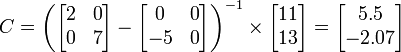 .
.
Now we have T and C and we can use them iteratively X matrices. So, now you will have x(1) = Tx(0) + C.
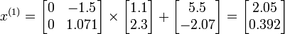 .
.
And now we can find x(2).
 .
.
Now you can test for convergence to see if you have found a set of possible solutions.
An example for the equation version
Suppose given k equations where xn are vectors of these equations and starting point x0. From the first equation solve for x1 in terms of xn + 1, xn + 2, ..., xn. For the next equations substitute the previous values of xs.
To make it clear let's consider an example.
- 10x1 − x2 + 2x3 = 6,
- − x1 + 11x2 − x3 + 3x4 = 25,
- 2x1 − x2 + 10x3 − x4 = − 11,
- 3x2 − x3 + 8x4 = 15.
Solving for x1, x2, x3 and x4 gives:
- x1 = x2 / 10 − x3 / 5 + 3 / 5,
- x2 = x1 / 11 + x3 / 11 − 3x4 / 11 + 25 / 11,
- x3 = − x1 / 5 + x2 / 10 + x4 / 10 − 11 / 10,
- x4 = − 3x2 / 8 + x3 / 8 + 15 / 8.
Suppose we choose (0,0,0,0) as the initial approximation, then the first approximate solution is given by
- x1 = 3 / 5 = 0.6,
- x2 = (3 / 5) / 11 + 25 / 11 = 3 / 55 + 25 / 11 = 2.3272,
- x3 = − (3 / 5) / 5 + (2.3272) / 10 − 11 / 10 = − 3 / 25 + 0.23272 − 1.1 = − 0.9873,
- x4 = − 3(2.3272) / 8 + ( − 0.9873) / 8 + 15 / 8 = 0.8789.
Using the approximations obtained, the iterative procedure is repeated until the desired accuracy has been reached. The following are the approximated solutions after four iterations.
| x1 | x2 | x3 | x4 |
|---|---|---|---|
| 0.6 | 2.32727 | − 0.987273 | 0.878864 |
| 1.03018 | 2.03694 | − 1.01446 | 0.984341 |
| 1.00659 | 2.00356 | − 1.00253 | 0.998351 |
| 1.00086 | 2.0003 | − 1.00031 | 0.99985 |
Multiple Choice Test: Gauss-Seidel Method of Solving Simultaneous Linear Equations

No comments:
Post a Comment